
Today we are going to see an another series of new product Spire.XLS which helps us to create, manipulate, convert EXCEL file to other formats, create charts dynamically and many more. This product has been introduced by the company E-Iceblue. I hope you have read my article of Spire.Doc and Spire.XLS. If you have not read it, I recommend you to read it here: Using Spire.XLS
Background
As you all know, charts are the graphical representations of our data. It is much easier to understand our data if it is in a graphical form. Am I right? It is easy to create a static chart, but what about a dynamic one? It will be bit tough right? But by using Spire.XLS, we can create any kind of charts easily. In this post, we will see those implementations.
Download the files
You can always get the needed files from here: Download Spire.XLS
Install Spire.XLS
I am using evaluation version with one month temporary license. There are free versions also available for spire.xls with some limitation. You can try that. Now click on the exe file after you extract the downloaded file. The installation will get started then.


Using the code
Before starting with coding you need to add the needed namespaces as follows.
[csharp]
using Spire.Xls;
using System.Drawing;
[/csharp]
First of all create a form and then a button, in the button click add the following lines of codes.
C# Code
[csharp]
private void button1_Click(object sender, EventArgs e)
{
try
{
//Create a new workbook
Workbook workbook = new Workbook();
//Initialize worksheet
workbook.CreateEmptySheets(1);
Worksheet sheet = workbook.Worksheets[0];
//Set sheet name
sheet.Name = "Chart data";
//Set the grid lines invisible
sheet.GridLinesVisible = false;
//Create a chart
Chart chart = sheet.Charts.Add(ExcelChartType.Pie3D);
//Set region of chart data
chart.DataRange = sheet.Range["B2:B5"];
chart.SeriesDataFromRange = false;
//Set position of chart
chart.LeftColumn = 1;
chart.TopRow = 6;
chart.RightColumn = 9;
chart.BottomRow = 25;
//Chart title
chart.ChartTitle = "Sales by year";
chart.ChartTitleArea.IsBold = true;
chart.ChartTitleArea.Size = 12;
//Initialize the chart series
Spire.Xls.Charts.ChartSerie cs = chart.Series[0];
//Chart Labels resource
cs.CategoryLabels = sheet.Range["A2:A5"];
//Chart value resource
cs.Values = sheet.Range["B2:B5"];
//Set the value visible in the chart
cs.DataPoints.DefaultDataPoint.DataLabels.HasValue = true;
//Year
sheet.Range["A1"].Value = "Year";
sheet.Range["A2"].Value = "2002";
sheet.Range["A3"].Value = "2003";
sheet.Range["A4"].Value = "2004";
sheet.Range["A5"].Value = "2005";
//Sales
sheet.Range["B1"].Value = "Sales";
sheet.Range["B2"].NumberValue = 4000;
sheet.Range["B3"].NumberValue = 6000;
sheet.Range["B4"].NumberValue = 7000;
sheet.Range["B5"].NumberValue = 8500;
//Style
sheet.Range["A1:B1"].Style.Font.IsBold = true;
sheet.Range["A2:B2"].Style.KnownColor = ExcelColors.LightYellow;
sheet.Range["A3:B3"].Style.KnownColor = ExcelColors.LightGreen1;
sheet.Range["A4:B4"].Style.KnownColor = ExcelColors.LightOrange;
sheet.Range["A5:B5"].Style.KnownColor = ExcelColors.LightTurquoise;
//Border
sheet.Range["A1:B5"].Style.Borders[BordersLineType.EdgeTop].Color = Color.FromArgb(0, 0, 128);
sheet.Range["A1:B5"].Style.Borders[BordersLineType.EdgeTop].LineStyle = LineStyleType.Thin;
sheet.Range["A1:B5"].Style.Borders[BordersLineType.EdgeBottom].Color = Color.FromArgb(0, 0, 128);
sheet.Range["A1:B5"].Style.Borders[BordersLineType.EdgeBottom].LineStyle = LineStyleType.Thin;
sheet.Range["A1:B5"].Style.Borders[BordersLineType.EdgeLeft].Color = Color.FromArgb(0, 0, 128);
sheet.Range["A1:B5"].Style.Borders[BordersLineType.EdgeLeft].LineStyle = LineStyleType.Thin;
sheet.Range["A1:B5"].Style.Borders[BordersLineType.EdgeRight].Color = Color.FromArgb(0, 0, 128);
sheet.Range["A1:B5"].Style.Borders[BordersLineType.EdgeRight].LineStyle = LineStyleType.Thin;
//Number format
sheet.Range["B2:C5"].Style.NumberFormat = "\"$\"#,##0";
chart.PlotArea.Fill.Visible = false;
//Save the file
workbook.SaveToFile("Sample.xls");
//Launch the file
System.Diagnostics.Process.Start("Sample.xls");
}
catch (Exception)
{
throw;
}
}
[/csharp]
VB.NET Code
[vb]
‘Create a new workbook
Dim workbook As New Workbook()
‘Initialize worksheet
workbook.CreateEmptySheets(1)
Dim sheet As Worksheet = workbook.Worksheets(0)
‘Set sheet name
sheet.Name = "Chart data"
‘Set the grid lines invisible
sheet.GridLinesVisible = False
‘Create a chart
Dim chart As Chart = sheet.Charts.Add(ExcelChartType.Pie3D)
‘Set region of chart data
chart.DataRange = sheet.Range("B2:B5")
chart.SeriesDataFromRange = False
‘Set position of chart
chart.LeftColumn = 1
chart.TopRow = 6
chart.RightColumn = 9
chart.BottomRow = 25
‘Chart title
chart.ChartTitle = "Sales by year"
chart.ChartTitleArea.IsBold = True
chart.ChartTitleArea.Size = 12
‘Set the chart
Dim cs As Spire.Xls.Charts.ChartSerie = chart.Series(0)
‘Chart Labels resource
cs.CategoryLabels = sheet.Range("A2:A5")
‘Chart value resource
cs.Values = sheet.Range("B2:B5")
‘Set the value visible in the chart
cs.DataPoints.DefaultDataPoint.DataLabels.HasValue = True
‘Year
sheet.Range("A1").Value = "Year"
sheet.Range("A2").Value = "2002"
sheet.Range("A3").Value = "2003"
sheet.Range("A4").Value = "2004"
sheet.Range("A5").Value = "2005"
‘Sales
sheet.Range("B1").Value = "Sales"
sheet.Range("B2").NumberValue = 4000
sheet.Range("B3").NumberValue = 6000
sheet.Range("B4").NumberValue = 7000
sheet.Range("B5").NumberValue = 8500
‘Style
sheet.Range("A1:B1").Style.Font.IsBold = True
sheet.Range("A2:B2").Style.KnownColor = ExcelColors.LightYellow
sheet.Range("A3:B3").Style.KnownColor = ExcelColors.LightGreen1
sheet.Range("A4:B4").Style.KnownColor = ExcelColors.LightOrange
sheet.Range("A5:B5").Style.KnownColor = ExcelColors.LightTurquoise
‘Border
sheet.Range("A1:B5").Style.Borders(BordersLineType.EdgeTop).Color = Color.FromArgb(0, 0, 128)
sheet.Range("A1:B5").Style.Borders(BordersLineType.EdgeTop).LineStyle = LineStyleType.Thin
sheet.Range("A1:B5").Style.Borders(BordersLineType.EdgeBottom).Color = Color.FromArgb(0, 0, 128)
sheet.Range("A1:B5").Style.Borders(BordersLineType.EdgeBottom).LineStyle = LineStyleType.Thin
sheet.Range("A1:B5").Style.Borders(BordersLineType.EdgeLeft).Color = Color.FromArgb(0, 0, 128)
sheet.Range("A1:B5").Style.Borders(BordersLineType.EdgeLeft).LineStyle = LineStyleType.Thin
sheet.Range("A1:B5").Style.Borders(BordersLineType.EdgeRight).Color = Color.FromArgb(0, 0, 128)
sheet.Range("A1:B5").Style.Borders(BordersLineType.EdgeRight).LineStyle = LineStyleType.Thin
‘Number format
sheet.Range("B2:C5").Style.NumberFormat = """$""#,##0"
chart.PlotArea.Fill.Visible = False
‘Save doc file.
workbook.SaveToFile("Sample.xls")
‘Launch the MS Word file.
System.Diagnostics.Process.Start("Sample.xls")
[/vb]
In the above lines code, we are creating a pie chart by giving some settings and data and load it. Now if you run you will get an output as follows.
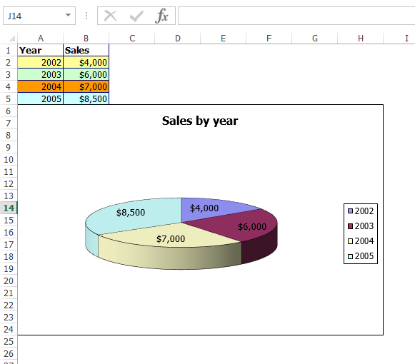
In the above mentioned lines of codes, we are doing so many processes, those processes are listed below.
Wow!. That’s cool right?
Not yet finished!. There are so many things you can try with your sheet object. I suggest you to try those. You will get surprised.
Working With Charts Using Spire XLS Sheet Object
Working With Charts Using Spire XLS Sheet Object
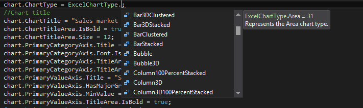
If you want you can set different chart types too, it will give you a great design in your chart. The most useful chart types which I uses is Bar3DClustered, 3DBubble, Bubble, Column3D and many more.
Working_With_Charts_Using_Spire_XLS_Chart_Object
This product gives you many ways to make your chart in the way you like. There are plenty of options available to so so like you can set the Legend Position by using LegendPositionType property.
Next we will see how we can implement Column chart, what ever we have discusses will be same for every charts, but it may have some different properties which is strictly depends on the chart type.
Column Chart
Now we will create an another button and name it Column Chart. And in the button click you need to add the following codes.
C# Code
[csharp]
private void button2_Click(object sender, EventArgs e)
{
try
{
//Load Workbook
Workbook workbook = new Workbook();
workbook.LoadFromFile(@"D:\Sample.xlsx");
Worksheet sheet = workbook.Worksheets[0];
//Add Chart and Set Chart Data Range
Chart chart = sheet.Charts.Add(ExcelChartType.ColumnClustered);
chart.DataRange = sheet.Range["D1:E17"];
chart.SeriesDataFromRange = false;
//Chart Position
chart.LeftColumn = 1;
chart.TopRow = 19;
chart.RightColumn = 8;
chart.BottomRow = 33;
//Chart Border
chart.ChartArea.Border.Weight = ChartLineWeightType.Medium;
chart.ChartArea.Border.Color = Color.SandyBrown;
//Chart Title
chart.ChartTitle = "Parts Sales Info";
chart.ChartTitleArea.Font.FontName = "Calibri";
chart.ChartTitleArea.Font.Size = 13;
chart.ChartTitleArea.Font.IsBold = true;
//Chart Axes
chart.PrimaryCategoryAxis.Title = "Parts";
chart.PrimaryCategoryAxis.Font.Color = Color.Blue;
chart.PrimaryValueAxis.Title = "Amounts";
chart.PrimaryValueAxis.HasMajorGridLines = false;
chart.PrimaryValueAxis.MaxValue = 350;
chart.PrimaryValueAxis.TitleArea.TextRotationAngle = 90;
//Chart Legend
chart.Legend.Position = LegendPositionType.Right;
//Save and Launch
workbook.SaveToFile("ExcelColumnChart.xlsx", ExcelVersion.Version2010);
System.Diagnostics.Process.Start("ExcelColumnChart.xlsx");
}
catch (Exception)
{
throw;
}
}
[/csharp]
VB.NET Code
[vb]
‘Load Workbook
Dim workbook As New Workbook()
workbook.LoadFromFile("E:\Sample.xlsx")
Dim sheet As Worksheet = workbook.Worksheets(0)
‘Add Chart and Set Chart Data Range
Dim chart As Chart = sheet.Charts.Add(ExcelChartType.ColumnClustered)
chart.DataRange = sheet.Range("D1:E17")
chart.SeriesDataFromRange = False
‘Chart Position
chart.LeftColumn = 1
chart.TopRow = 19
chart.RightColumn = 8
chart.BottomRow = 33
‘Chart Border
chart.ChartArea.Border.Weight = ChartLineWeightType.Medium
chart.ChartArea.Border.Color = Color.SandyBrown
‘Chart Title
chart.ChartTitle = "Parts Sales Info"
chart.ChartTitleArea.Font.FontName = "Calibri"
chart.ChartTitleArea.Font.Size = 13
chart.ChartTitleArea.Font.IsBold = True
‘Chart Axes
chart.PrimaryCategoryAxis.Title = "Parts"
chart.PrimaryCategoryAxis.Font.Color = Color.Blue
chart.PrimaryValueAxis.Title = "Amounts"
chart.PrimaryValueAxis.HasMajorGridLines = False
chart.PrimaryValueAxis.MaxValue = 350
chart.PrimaryValueAxis.TitleArea.TextRotationAngle = 90
‘Chart Legend
chart.Legend.Position = LegendPositionType.Right
‘Save and Launch
workbook.SaveToFile("ExcelColumnChart.xlsx", ExcelVersion.Version2010)
System.Diagnostics.Process.Start("ExcelColumnChart.xlsx")
[/vb]
Now if you run the code, you can see an output as follows.
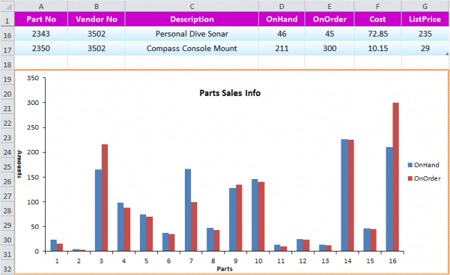
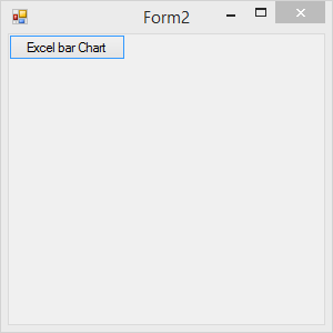
Excel Bar Chart
Before going through you must add an new namespace as follows.
[csharp]
using Spire.Xls.Charts;
[/csharp]
Now we will create an another button in our form and in the click event we will write the receding lines of codes.
[csharp]
private void button1_Click(object sender, EventArgs e)
{
try
{
Workbook workbook = new Workbook();
//Initailize worksheet
workbook.CreateEmptySheets(1);
Worksheet sheet = workbook.Worksheets[0];
sheet.Name = "Chart data";
sheet.GridLinesVisible = false;
//Writes chart data
CreateChartData(sheet);
//Add a new chart worsheet to workbook
Chart chart = sheet.Charts.Add();
//Set region of chart data
chart.DataRange = sheet.Range["A1:C5"];
chart.SeriesDataFromRange = false;
//Set position of chart
chart.LeftColumn = 1;
chart.TopRow = 6;
chart.RightColumn = 11;
chart.BottomRow = 29;
chart.ChartType = ExcelChartType.Bar3DClustered;
//Chart title
chart.ChartTitle = "Sales market by country";
chart.ChartTitleArea.IsBold = true;
chart.ChartTitleArea.Size = 12;
chart.PrimaryCategoryAxis.Title = "Country";
chart.PrimaryCategoryAxis.Font.IsBold = true;
chart.PrimaryCategoryAxis.TitleArea.IsBold = true;
chart.PrimaryCategoryAxis.TitleArea.TextRotationAngle = 90;
chart.PrimaryValueAxis.Title = "Sales(in Dollars)";
chart.PrimaryValueAxis.HasMajorGridLines = false;
chart.PrimaryValueAxis.MinValue = 1000;
chart.PrimaryValueAxis.TitleArea.IsBold = true;
foreach (ChartSerie cs in chart.Series)
{
cs.Format.Options.IsVaryColor = true;
cs.DataPoints.DefaultDataPoint.DataLabels.HasValue = true;
}
chart.Legend.Position = LegendPositionType.Top;
workbook.SaveToFile("Sample.xls");
ExcelDocViewer(workbook.FileName);
}
catch (Exception)
{
throw;
}
}
[/csharp]
As you can see we are calling a function CreateChartData to generate the data, so now we will write the function body.
[csharp]
private void CreateChartData(Worksheet sheet)
{
//Country
sheet.Range["A1"].Value = "Country";
sheet.Range["A2"].Value = "Cuba";
sheet.Range["A3"].Value = "Mexico";
sheet.Range["A4"].Value = "France";
sheet.Range["A5"].Value = "German";
//Jun
sheet.Range["B1"].Value = "Jun";
sheet.Range["B2"].NumberValue = 6000;
sheet.Range["B3"].NumberValue = 8000;
sheet.Range["B4"].NumberValue = 9000;
sheet.Range["B5"].NumberValue = 8500;
//Jun
sheet.Range["C1"].Value = "Aug";
sheet.Range["C2"].NumberValue = 3000;
sheet.Range["C3"].NumberValue = 2000;
sheet.Range["C4"].NumberValue = 2300;
sheet.Range["C5"].NumberValue = 4200;
//Style
sheet.Range["A1:C1"].Style.Font.IsBold = true;
sheet.Range["A2:C2"].Style.KnownColor = ExcelColors.LightYellow;
sheet.Range["A3:C3"].Style.KnownColor = ExcelColors.LightGreen1;
sheet.Range["A4:C4"].Style.KnownColor = ExcelColors.LightOrange;
sheet.Range["A5:C5"].Style.KnownColor = ExcelColors.LightTurquoise;
//Border
sheet.Range["A1:C5"].Style.Borders[BordersLineType.EdgeTop].Color = Color.FromArgb(0, 0, 128);
sheet.Range["A1:C5"].Style.Borders[BordersLineType.EdgeTop].LineStyle = LineStyleType.Thin;
sheet.Range["A1:C5"].Style.Borders[BordersLineType.EdgeBottom].Color = Color.FromArgb(0, 0, 128);
sheet.Range["A1:C5"].Style.Borders[BordersLineType.EdgeBottom].LineStyle = LineStyleType.Thin;
sheet.Range["A1:C5"].Style.Borders[BordersLineType.EdgeLeft].Color = Color.FromArgb(0, 0, 128);
sheet.Range["A1:C5"].Style.Borders[BordersLineType.EdgeLeft].LineStyle = LineStyleType.Thin;
sheet.Range["A1:C5"].Style.Borders[BordersLineType.EdgeRight].Color = Color.FromArgb(0, 0, 128);
sheet.Range["A1:C5"].Style.Borders[BordersLineType.EdgeRight].LineStyle = LineStyleType.Thin;
sheet.Range["B2:C5"].Style.NumberFormat = "\"$\"#,##0";
}
[/csharp]
And we will use the preceding function for viewing our chart created.
[csharp]
private void ExcelDocViewer(string fileName)
{
try
{
System.Diagnostics.Process.Start(fileName);
}
catch { }
}
[/csharp]
Now it is time to run our program. You will see the output as follows.
Excel Bar Chart
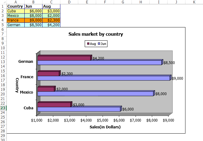
Excel Bar Chart
As you can see it is very easy to give styles and border to our chart.
[csharp]
//Style
sheet.Range["A1:C1"].Style.Font.IsBold = true;
sheet.Range["A2:C2"].Style.KnownColor = ExcelColors.LightYellow;
sheet.Range["A3:C3"].Style.KnownColor = ExcelColors.LightGreen1;
sheet.Range["A4:C4"].Style.KnownColor = ExcelColors.LightOrange;
sheet.Range["A5:C5"].Style.KnownColor = ExcelColors.LightTurquoise;
//Border
sheet.Range["A1:C5"].Style.Borders[BordersLineType.EdgeTop].Color = Color.FromArgb(0, 0, 128);
sheet.Range["A1:C5"].Style.Borders[BordersLineType.EdgeTop].LineStyle = LineStyleType.Thin;
sheet.Range["A1:C5"].Style.Borders[BordersLineType.EdgeBottom].Color = Color.FromArgb(0, 0, 128);
sheet.Range["A1:C5"].Style.Borders[BordersLineType.EdgeBottom].LineStyle = LineStyleType.Thin;
sheet.Range["A1:C5"].Style.Borders[BordersLineType.EdgeLeft].Color = Color.FromArgb(0, 0, 128);
sheet.Range["A1:C5"].Style.Borders[BordersLineType.EdgeLeft].LineStyle = LineStyleType.Thin;
sheet.Range["A1:C5"].Style.Borders[BordersLineType.EdgeRight].Color = Color.FromArgb(0, 0, 128);
sheet.Range["A1:C5"].Style.Borders[BordersLineType.EdgeRight].LineStyle = LineStyleType.Thin;
sheet.Range["B2:C5"].Style.NumberFormat = "\"$\"#,##0";
[/csharp]
Like this we can crate Line Chart, Radar Chart and many more. Please try those too. Now we will see How to Save Excel Charts as Images.
How to Save Excel Charts as Images
Create another button and write the preceding codes in button click.
[csharp]
private void button2_Click(object sender, EventArgs e)
{
Workbook workbook = new Workbook();
workbook.LoadFromFile("D:\\Sample.xlsx", ExcelVersion.Version2010);
Worksheet sheet = workbook.Worksheets[0];
Image[] imgs = workbook.SaveChartAsImage(sheet);
for (int i = 0; i < imgs.Length; i++)
{
imgs[i].Save(string.Format("img-{0}.png", i), System.Drawing.Imaging.ImageFormat.Png);
}
}
[/csharp]
Here we are taking a file called Sample.xlsx and loop through the charts inside the file and save those as images with few lines codes. Sounds good right?
VB.Net Code
[vb]
Dim workbook As New Workbook()
workbook.LoadFromFile("D:\\Sample.xlsx", ExcelVersion.Version2010)
Dim sheet As Worksheet = workbook.Worksheets(0)
Dim imgs As Image() = workbook.SaveChartAsImage(sheet)
For i As Integer = 0 To imgs.Length – 1
imgs(i).Save(String.Format("img-{0}.png", i), ImageFormat.Png)
Next
[/vb]
Conclusion
I hope you liked this article. Please share me your valuable suggestions and feedback.
Kindest Regards
Sibeesh Venu